The Equation That Landed on the Moon

In the autumn of 1960, a mathematician named Rudolf Kalman walked into NASA’s Ames Research Center and met an engineer named Stanley Schmidt. Schmidt’s team had a problem that sounds impossible: figure out where a spacecraft is, on the way to the Moon, using a few noisy measurements and a computer with less memory than a modern doorbell.

Kalman had just published a filter for exactly this kind of “estimate the truth from noisy data” problem. Schmidt realised it could be bent to handle the nonlinear math of spaceflight, and the version his team built (later called the Extended Kalman Filter) ended up running on the Apollo Guidance Computer. It did not single-handedly land anyone on the Moon, that took a lot more than one equation, but it is fair to say the Kalman filter is what made Apollo’s navigation actually practical.

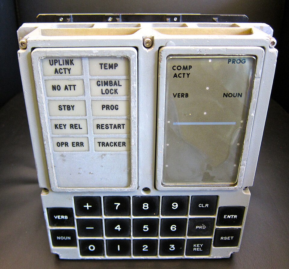the DSKY, the display and keypad astronauts used to drive the Apollo Guidance Computer. somewhere behind it, a Kalman filter was fusing noisy measurements into a trajectory. photo by Steve Jurvetson, Wikimedia Commons, CC BY 2.0

That keypad is how the astronauts actually talked to the computer, by punching in VERB and NOUN codes (you can see both labels on the right panel). No graphics, no mouse, just a calculator-style box. And behind that little display it was doing exactly what this post is about: taking noisy star sightings and radar ranges and folding them into one best guess of where the spacecraft was. The same predict-then-correct loop my drone runs, just aimed at the Moon instead of my room.

Sixty years later, the same family of math runs on my little drone simulator, 200 times a second. And it is the answer to the exact question I left hanging at the end of last post: if the gyro lies one way and the accelerometer lies another, how does the drone ever figure out the truth?

Where we are in the series. Frames, quaternions, dynamics, and sensors. Today we fuse those sensors into one estimate the drone can actually trust. This is the hardest post so far, so take it slow.

The Big Idea: Guess, Then Correct

Here is the whole Kalman filter in one sentence, before any math: make a guess, then correct it with a measurement, and repeat forever.

That is it. The filter runs a loop with two steps:

1. Predict. Use what you know about how the system moves to guess where it is now. For my drone, that means “the gyro says I rotated this much since last time, so my new orientation is probably this.”
2. Correct. Take a real measurement and nudge your guess toward it. “The accelerometer says down is over there, and that disagrees a little with my guess, so let me shift my guess partway toward it.”

Then the corrected estimate becomes the starting point for the next prediction, and round it goes.

You already do this. Walking through a dark room you have lived in for years, you predict where the doorway is from memory, then correct with your hand when you brush the wall. Predict from a model, correct with a measurement. The Kalman filter just does it with numbers, and does it in the mathematically optimal way.

Here is the loop drawn out properly:

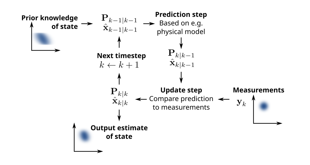one full cycle of a Kalman filter. it carries two things round the loop: the estimate (x-hat) and how unsure it is (P). predict pushes both forward in time, the update step pulls them toward a fresh measurement. figure by Petteri Aimonen, Wikimedia Commons, public domain

Notice the diagram carries two things around the loop, not one. There is the estimate itself, and there is a little blurry cloud around it. That cloud is the important part, so let me talk about it.

Trust Is Just a Number

The thing that makes a Kalman filter special, the reason it beats just averaging your sensors, is that it keeps track of how unsure it is.

At every moment the filter holds two things:

• its best estimate (say, the drone’s orientation), and
• a number for how much it trusts that estimate, called the covariance, written $P$.

Small $P$ means “I am very sure”. Big $P$ means “I am guessing, do not quote me”. And $P$ is alive, it changes every step. When the filter predicts, $P$ grows (guessing makes you less sure). When it folds in a good measurement, $P$ shrinks (you just learned something).

Now the actual magic. When a new measurement arrives, the filter has two opinions about the world: its own prediction, and the measurement. Each comes with its own uncertainty. So which do you believe? The answer is simple: lean more toward the one you trust more. The number that strikes that balance is called the Kalman gain.

If that sounds abstract, it is about to become concrete, because the cleanest way to actually feel how $P$ and the gain work is to throw away all the matrices and do the whole thing with a single number.

The 1D Warm-Up (This Is The Important Bit)

Forget quaternions. Forget the drone, almost. Let us estimate just one number: the drone’s tilt, in one direction, as a single angle. Call it $\theta$.

We have the same two sources from last post:

• the gyro, which tells us the rotation rate, so we can predict how $\theta$ changes, and
• the accelerometer, which gives us a noisy direct measurement of $\theta$ (it knows where “down” is).

The filter keeps two numbers: our estimate $\hat{\theta}$, and our uncertainty $P$ (one number now, not a matrix). Watch how four little update rules give us the entire Kalman filter.

Step 1: Predict

The gyro says we rotated at rate $\omega$ for a time step $dt$, so our new angle is probably:

\[\hat{\theta} \leftarrow \hat{\theta} + \omega \, dt\]

But the gyro is noisy (it has that random walk from last post), so this prediction is a bit shakier than what we started with. We bump up our uncertainty:

\[P \leftarrow P + Q\]

$Q$ is “how much trust we lose per prediction”, and it comes straight from the gyro’s noise spec. Noisy gyro, big $Q$, uncertainty grows fast. This is the filter being honest: every guess makes it a little less sure.

Step 2: Correct

Now the accelerometer hands us a measurement $z$ of the angle. It disagrees with our prediction by some amount. That disagreement has a name, the innovation:

\[\text{innovation} = z - \hat{\theta}\]

How much should we move our estimate toward the measurement? That is the Kalman gain $K$:

\[K = \frac{P}{P + R}\]

where $R$ is how noisy we believe the accelerometer is (also from last post’s specs). Look at what this little fraction does, because it is the whole filter:

• If the accelerometer is very noisy ($R$ huge), then $K \to 0$. We basically ignore the measurement and keep our prediction.
• If our own prediction is very shaky ($P$ huge), then $K \to 1$. We throw out our guess and jump to the measurement.
• Normally it sits somewhere between, a weighted blend.

$K$ is literally “how much do I trust the new measurement versus myself”, as a number between 0 and 1. Then we apply it:

\[\hat{\theta} \leftarrow \hat{\theta} + K \, (z - \hat{\theta})\]

and, because we just learned something, our uncertainty shrinks:

\[P \leftarrow (1 - K)\, P\]

That is the entire Kalman filter. Four lines. Predict the value and grow $P$, then compute the gain, correct the value and shrink $P$. Loop forever.

Everything from here on, the matrices, the “Extended”, the “Multiplicative”, is just this same four-line idea, expanded to handle 3D rotations instead of one cosy little angle. If those four lines make sense, you have already understood 80% of what runs on my drone. Genuinely, this is the part I had to sit with for a few days before it clicked, so if it has not clicked yet, reread this section and not the scary ones below.

Why “Extended”?

Our 1D toy had a lovely property: everything was a straight line. Predicting was just addition. Measuring was just reading off the angle. When all the relationships are linear, the plain Kalman filter is exactly, provably optimal.

Real life is not a straight line. On the actual drone, the accelerometer does not measure orientation directly. It measures gravity in the body frame, and getting from “my orientation” to “which way gravity points in my body frame” means rotating a vector through a quaternion, which is very much not linear (it is full of products and squares of the quaternion components, as we saw in the quaternion post).

The fix is the move Stanley Schmidt made for Apollo: at each step, pretend the curve is a straight line just near where you currently are. Zoom in close enough on any smooth curve and it looks straight. So the filter takes the nonlinear relationship, computes its slope at the current best estimate, and uses that straight-line approximation for one step. Next step, it re-zooms at the new estimate. That local “slope of a multi-variable function” is called the Jacobian, and a Kalman filter that linearizes this way is the Extended Kalman filter (EKF). That is the whole upgrade: linearize the curvy bits, fresh each step.

Why “Multiplicative”? (The Part That Trips People Up)

In the 1D toy, correcting was easy: just add a little bit to the angle, $\hat{\theta} \leftarrow \hat{\theta} + \text{something}$. But you cannot do that with a quaternion. Quaternions have to stay unit length to be valid rotations (quaternion post), and if you just add a correction to the four numbers, you knock it off the unit sphere and it stops being a rotation at all.

So the MEKF (Multiplicative Extended Kalman Filter) does something clever, and here is the whole idea in one plain sentence:

We do not add a correction directly to the quaternion. Instead we estimate a tiny 3D rotation error, multiply it into the quaternion, and then reset the error back to zero.

That is what the M, multiplicative, means. The filter does not track the orientation as its state to be corrected. It tracks a small error: “how far off is my current quaternion, expressed as a tiny rotation?” That error is just a little 3-number rotation (call it $\delta\theta$), and small rotations do live in nice flat space where the ordinary Kalman math works. Once the filter computes the error, it applies it to the quaternion by multiplication (which keeps it unit length, because multiplying unit quaternions gives a unit quaternion), and then sets the error back to zero, ready to accumulate again.

This is the error state. On my drone the filter actually tracks six error numbers:

\[\delta x = [\,\underbrace{\delta\theta}_{\text{3 attitude error}},\ \underbrace{\delta b}_{\text{3 gyro bias error}}\,]\]

The first three are the small attitude error we just described. The other three are the error in our estimate of the gyro’s bias, because remember from last post, the gyro has a slowly drifting bias, and a great bonus of this filter is that it actually estimates and removes that bias for free as it runs. That is huge: the filter is not just smoothing the gyro, it is learning the gyro’s systematic lie and subtracting it.

Now we have all the ideas. Predict and correct, track uncertainty $P$, weight by the Kalman gain, linearize the nonlinear bits (Extended), and correct rotations by a small multiplied-in error (Multiplicative). The rest is just seeing it in my code.

How My Code Actually Does It

The filter lives in mekf_node.cpp. It subscribes to the raw IMU and publishes a clean orientation estimate. The state is exactly what we described:

Vec4 q_;   // attitude quaternion (w,x,y,z)
Vec3 b_;   // gyro bias estimate
Mat6 P_;   // 6x6 uncertainty (3 attitude error + 3 bias error)
Mat6 Q_;   // process noise (how much trust we lose predicting)
Mat3 R_accel_; // accelerometer noise (how much we trust the measurement)

And Q_ and R_accel_ are built directly from the ADIS16470 noise specs from last post, so the filter’s idea of “how much to trust each sensor” is calibrated to the real datasheet, not guessed.

Predict, in code

Exactly the 1D predict step, just in 3D. Subtract the estimated bias from the gyro, integrate it into the quaternion, then grow the covariance:

void predict(const Vec3& omega_raw)
{
    Vec3 w = omega_raw - b_;     // remove the bias we have learned
    q_ = qintegrate(q_, w, DT);  // gyro pushes the orientation forward

    Mat6 Phi = Mat6::Identity();
    Phi.block<3,3>(0,0) -= skew(w) * DT;
    Phi.block<3,3>(0,3)  = -Mat3::Identity() * DT;
    P_ = Phi * P_ * Phi.transpose() + Q_;   // P <- P + Q, the 3D version
}

That last line is P <- P + Q from the toy, wearing matrices. The + Q_ is the same “we just guessed, trust ourselves a little less” bump.

Correct, in code

And this is the 1D correct step in 3D. Work out where the filter thinks gravity should point in the body frame, compare to what the accelerometer actually read (the innovation), compute the gain, apply the correction:

Vec3 g_body = qR(q_).transpose() * Vec3(0, 0, GRAVITY);  // predicted gravity
Vec3 y = accel - g_body;                                 // innovation: measured - predicted

Mat3 S = H * P_ * H.transpose() + R_accel_;   // S = P + R, the denominator
Eigen::Matrix<double,6,3> K = P_ * H.transpose() * S.inverse();  // Kalman gain

Vec6 dx = K * y;     // the error state: how wrong are we?

Compare K = P_ * H.transpose() * S.inverse() to the toy’s $K = P / (P+R)$. Same fraction, “my uncertainty over total uncertainty”, just with matrices and the Jacobian H doing the linearizing. And dx = K * y is K * (z - prediction) from the toy.

Then the multiplicative bit. The error dx splits into the attitude error and the bias error, and we apply each:

Vec3 dtheta = dx.head<3>();                  // small rotation error
Vec4 dq(1.0, dtheta[0]/2, dtheta[1]/2, dtheta[2]/2);
q_ = qnorm(qmul(q_, dq));   // MULTIPLY the error in, then renormalize

b_ += dx.tail<3>();         // nudge the bias estimate too

There it is: q_ = qmul(q_, dq), the quaternion gets the error multiplied in, not added, and qnorm keeps it unit length. The error is applied and effectively reset. That single line is the entire reason this is an MEKF and not a regular EKF.

Don’t Trust the Accelerometer Mid-Maneuver

Here is my favourite line in the whole filter, because it keeps the filter honest:

if (std::abs(accel.norm() - GRAVITY) > 2.0) return;

Remember the catch from last post: an accelerometer only reads pure gravity when the drone is not accelerating hard. The second the drone yanks itself sideways, the accelerometer feels that thrust too, and “down” is no longer where gravity is. So if the measured acceleration is more than 2 m/s² away from a clean $1g$, the filter knows the accelerometer is currently lying extra, and it just skips the correction and coasts on the gyro until things calm down. It refuses to listen to a measurement it knows is bad right now.

Tiny sidebar, the Joseph form. The covariance update on the last line of correct() is written in a longer-than-necessary way ((I - KH) P (I - KH)^T + K R K^T). That specific arrangement, the Joseph form, is just the numerically stable way to write it, so floating-point rounding can never make $P$ go invalid. Not conceptually deep, but it is why the filter does not quietly break after a few minutes. File under “boring things that matter”.

So, How Does a Drone Trust Two Liars?

It does not trust either one. It tracks how much to trust each, moment to moment, and blends them by exactly that amount. The gyro carries the estimate smoothly between measurements, the accelerometer reins in the gyro’s drift whenever it is safe to listen, and the filter quietly learns the gyro’s bias along the way. Two unreliable sensors, one estimate you can actually fly on.

The big picture to walk away with:

• A Kalman filter is just predict, then correct, forever, while tracking how unsure it is ($P$).
• The Kalman gain is the trust dial: it weights prediction against measurement by their uncertainties. The four-line 1D toy is the whole filter.
• Extended means we linearize the nonlinear bits fresh each step, the Apollo trick.
• Multiplicative means we correct the quaternion with a small rotation error multiplied in, never added, so it stays a valid rotation. And we get gyro bias estimation for free.
• The filter is honest enough to ignore the accelerometer during hard maneuvers.

And now, finally, the drone knows which way is up, reliably, even while moving. Which unlocks the last big question of this whole series: given where the drone is and where it wants to go, how does it actually command four motors to get there? That is the control problem, and PID is the answer. Next post.

Further Reading

• NASA TM 86847, Discovery of the Kalman Filter as a Practical Tool for Aerospace and Industry, the actual NASA history of how Schmidt’s team adapted the filter for Apollo. A lovely read.
• Joan Solà, Quaternion Kinematics for the Error-State Kalman Filter, the gold-standard derivation of everything in this post, done properly. Heavy but worth it if you want to build your own.

Thanks for reading. NASA trusted this thing to find the Moon, I am just trusting it to find which way is up, so if I got anything wrong pls ping me on X and I will fix it.